Stippling pictures with Lloyd's algorithm
(The MATLAB code can be found here)
When I was doing my project about inverting proton radiograms and shadowgrams, I discovered that the technique I employed can be used to make stipple pictures. The stippling technique I explained below comes from this paper.
What is stippling?
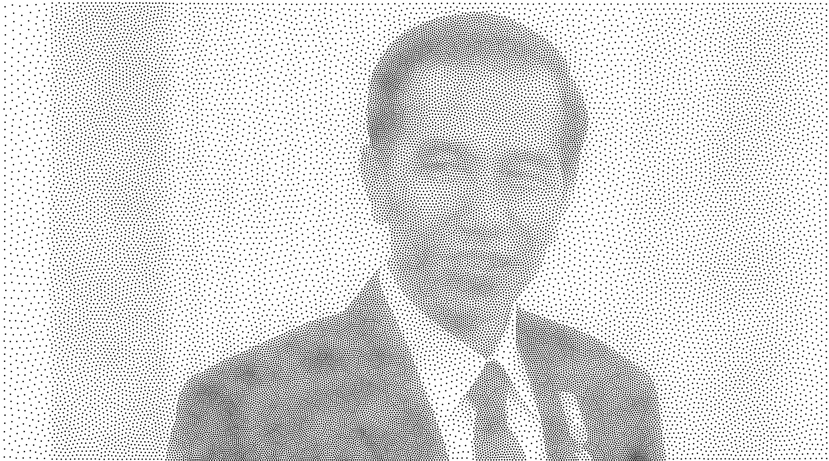
Stippling is a technique to produce a picture using small dots. The picture shown on top of this post is one of the example of stippling. At far, it looks like a common gray picture, but if you look at it closely, it is actually resembled of small dots. Look at picture below (click for the full size picture).
The picture above is the stippled picture of Presiden Jokowi generated using weighted Lloyd’s algorithm. The source is from Kemendagri website. Before I am going to explain about Lloyd’s algorithm, it is better to know about Voronoi diagram first.
Voronoi diagram
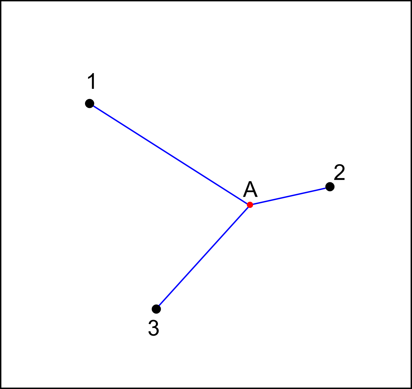
Consider a 2D plane and there are several dots on the plane. Now we are going to determine for all positions on the plane, which dot is the closest. For example in the picture below, point A is the closest to the dot 2, compared to the other dots. So in this case, point A belongs to dot 2.
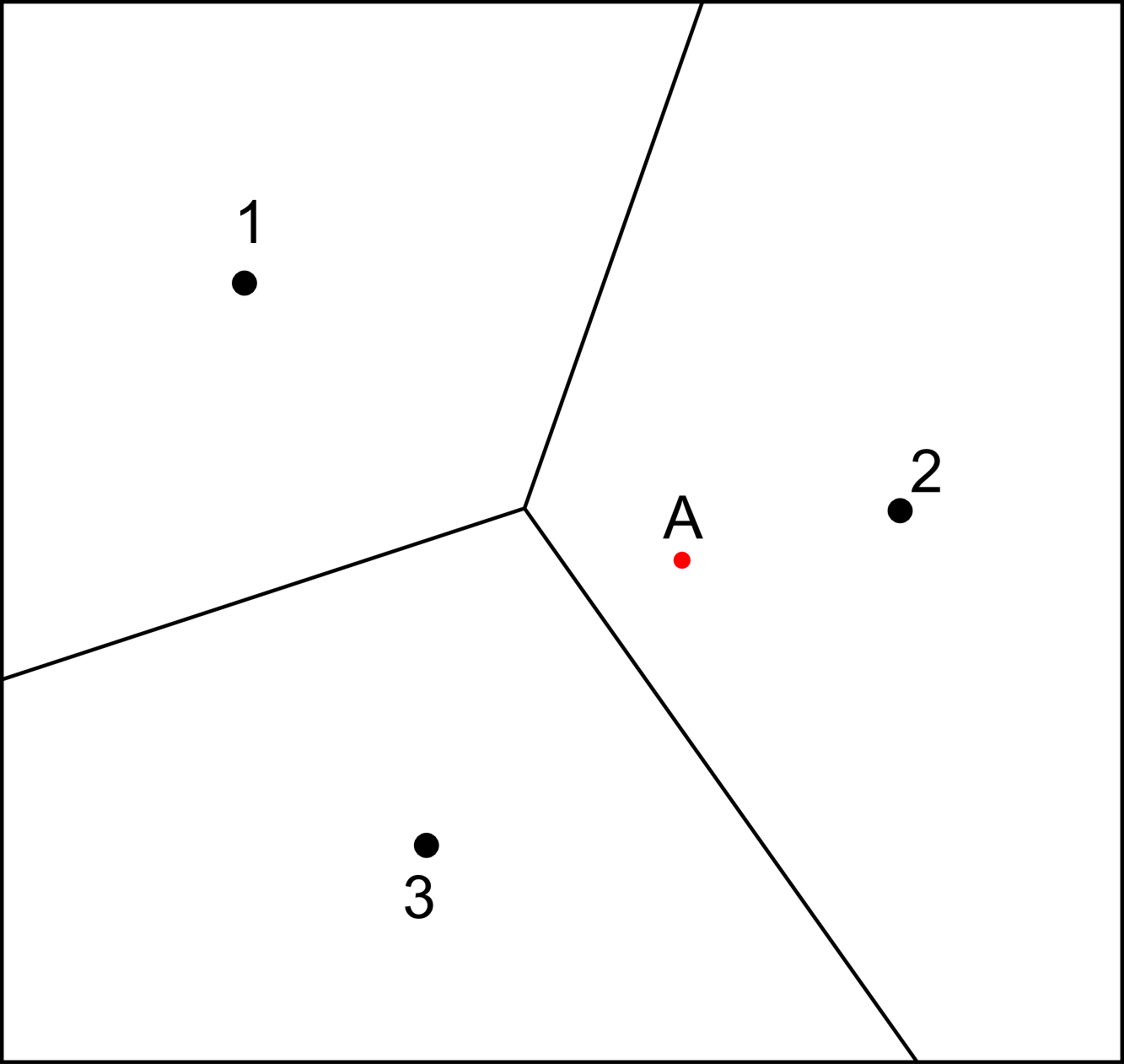
In construction of Voronoi diagram, we don’t consider one point only, but we consider all (continuous) points on the plane. After determining which dot is the closest to each points on the plane, we can draw borders between the dots to divide the plane into several regions or known as Voronoi cells. All points inside one cell belongs to the dot in the same cell. The result is a Voronoi diagram.
There have been a lot of libraries for various programming languages to construct Voronoi cell, so we don’t need to implement the algorithm by ourselves.
Lloyd’s algorithm
For a bounded plane, Lloyd’s algorithm is an algorithm to divide the plane into several regions with approximately the same size. The algorithm is simple:
- We start by deploying several dots on the plane randomly.
- Construct the Voronoi diagram inside the bounded plane.
- Calculate the centroid of each cell.
- Move the dots to its cell’s centroids.
- Repeat from step 2 until any stopping conditions fulfilled.
Here is a nice illustration of Lloyd’s algorithm from Wikipedia.
A Voronoi cell is always a convex polygon. Therefore, the formula of computing the centroid is quite straightforward. It is given by
\[C_x = \frac{1}{6A} \sum_{i=0}^{n-1} \left(x_i + x_{i+1}\right)\left(x_i y_{i+1} - x_{i+1} y_i\right)\] \[C_y = \frac{1}{6A} \sum_{i=0}^{n-1} \left(y_i + y_{i+1}\right)\left(x_i y_{i+1} - x_{i+1} y_i\right)\]where the area, \( A \) is
\[A = \frac{1}{2} \sum_{i=0}^{n-1} \left(x_i y_{i+1} - x_{i+1} y_i\right).\]The coordinates, \( (x_i, y_i) \), appear in counter-clockwise order and \( (x_n, y_n) = (x_0, y_0) \). Multiplication of the centroid position and the area is called as the first moment of the area.
Weighted Lloyd’s algorithm
So far, we only consider a uniform plane, without any particular weights at particular positions. How about the plane is not uniformly weighted so that the dots prefer to move to area with higher weight? If this is the case, the steps on Lloyd’s algorithm given above does not change. The only thing that changes is on how we calculate the centroid of each cell.
If the weight is given in pixels (i.e. uniform weight for a given square region), each cell is clipped by every pixel it touches. Then we calculate the first moment and area of each clipped region. To get the total first moment and area of the cell, we can sum all first moments and area from every clipped regions, respectively. Thus, the centroid position is simply the first moment divided by the total area.
Let’s denote superscript \(\ ^{(j)}\) as the property of the \(j\)-th clipped region within a cell. The weight of the clipped region is given by \(w^{(j)}\). The first moment and area of the region are given by
\[S_x^{(j)} = \frac{1}{6} w^{(j)} \sum_{i=0}^{n-1} \left(x_i^{(j)} + x_{i+1}^{(j)}\right)\left(x_i^{(j)} y_{i+1}^{(j)} - x_{i+1}^{(j)} y_i^{(j)}\right)\] \[S_y^{(j)} = \frac{1}{6} w^{(j)} \sum_{i=0}^{n-1} \left(y_i^{(j)} + y_{i+1}^{(j)}\right)\left(x_i^{(j)} y_{i+1}^{(j)} - x_{i+1}^{(j)} y_i^{(j)}\right)\] \[A^{(j)} = \frac{1}{2} w^{(j)} \sum_{i=0}^{n-1} \left(x_i^{(j)} y_{i+1}^{(j)} - x_{i+1}^{(j)} y_i^{(j)}\right).\]Thus, the centroid of the cell is given by
\[C_x = \frac{1}{A} \sum_{j=0}^{m-1} S_x^{(j)}\] \[C_y = \frac{1}{A} \sum_{j=0}^{m-1} S_y^{(j)}\]where the total area is
\[A = \sum_{j=0}^{m-1} A^{(j)}.\]To clip the cell with each pixel efficiently, I am using Sutherland-Hodgman algorithm.
Stippling with weighted Lloyd’s algorithm
From here, the things become relatively straightforward. The first step to do stippling for an image is to convert the image into grayscale image. One problem with the grayscale image is that darker regions have lower pixel values/weights and brighter regions have higher weights. On the other hand, we want more dots in darker regions and less dots in brighter regions. The solution is just to take the complement of the image.
Once the complement is taken, we can deploy random dots on the image and perform the weighted Lloyd’s algorithm. To make it converge faster, I used simple rejection method when deploying the random dots. The dots deployed in higher weight regions get more chance to be accepted. If a dot is rejected, then it must be deployed somewhere else. For most cases, repeating the iterations in the weighted Lloyd’s algorithm 50 times should be enough.
For those who want to try stippling their images, I have uploaded my MATLAB code in GitHub. Feel free to give your thought below.


