Bayesian Inverse Problem
Over the Easter holiday last week, I challenged myself to derive the posterior of Bayesian inverse problem. In easier terms, let’s say I have an unknown object enclosed inside a black box. Unfortunately, I can see the object from limited directions only (let’s say there are 3 small holes on the box). From the observations, I want to know what the full shape of the object. This is called as an inverse problem.
There are a lot of tools in solving the inverse problem, including where the number of observations are limited (like our example case) with reasonable assumptions on the object (e.g. the object is smooth). However, these tools only cannot answer some questions, like:
- How confident you are with your answer?
- Which part of the object that you are most confident and which part you are least confident?
- If you are free to choose the holes location on the box (but you can only make 3 small holes), where should you choose? Answering these questions need an additional approach from Bayesian inference, thus Bayesian inverse problem.
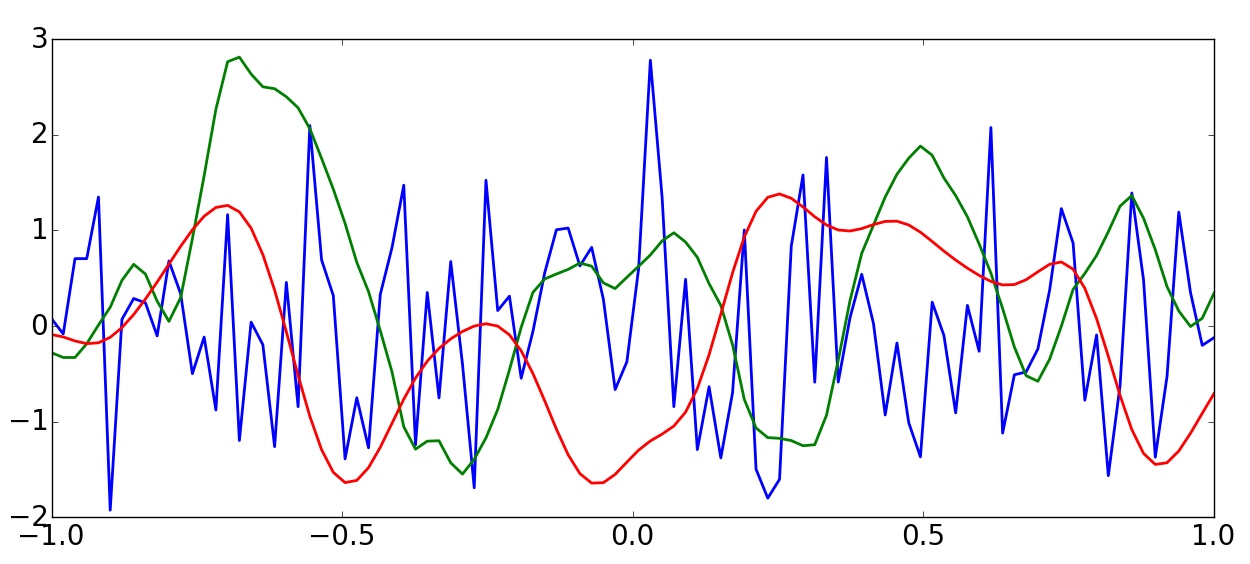
My first starting point was Gaussian Process (GP). In GP, it is assumed that interesting signals/functions are smooth to certain extent. Let’s take a look on the figure below. Most interesting signals/functions would have shape similar to the red line or green line. It is rarely to make the function in blue line interesting (unless you are interested in noise).
Based on the assumption, we can say that the values of a function \(f(x)\) is correlated for nearby points. If \(f(0) = 1\), then it is more likely for \(f(0.01)\) to have value close to 1. The correlation of two function values at \(x\) and \(x’\) is expressed in a kernel, \(k(x, x’)\). You can see choice of kernel functions from the Wikipedia of Gaussian Process. Statistically, the values of a function at several points, \(x_1, …, x_t \), is a random multivariate variables with distribution
\[\begin{equation} P(\mathbf{f}) = \mathcal{N}\left[0, \mathbf{K} \right] \propto \exp\left(\mathbf{f}^T\mathbf{K}^{-1}\mathbf{f}\right) \end{equation}\]where \(\mathbf{f}\) is just a vector of function values at several points, \(\mathcal{N}\) is the Normal distribution and \(\mathbf{K}\) is the covariance matrix with the element \(\mathbf{K}_{ij} = k(x_i, x_j) \).
Now let’s say we make an indirect observation, \(\mathbf{y} = \mathbf{Sf}\). We know our observation result, \(\mathbf{y}\), our observation method, \(\mathbf{S}\), and we want to infer what \(\mathbf{f}\) look like. This is an inference problem where we want to know the posterior distribution of \(\mathbf{f}\) after knowing \(\mathbf{y}\), i.e. \(P(\mathbf{f}|\mathbf{y})\). The posterior distribution can be derived from Bayesian theorem,
\[\begin{equation} P(\mathbf{f}|\mathbf{y}) = \frac{P(\mathbf{f},\mathbf{y})}{P(\mathbf{y})}. \end{equation}\]In the equation above, we know neither \(P(\mathbf{f},\mathbf{y})\) nor \(P(\mathbf{y})\). Fortunately, Normal distribution is very convenient with linear transformation. If the vector \(\mathbf{f}\) is multiplied by a matrix \(\mathbf{S}\), then the distribution becomes
\[\begin{equation} P(\mathbf{Sf}) = \mathcal{N}\left[0, \mathbf{SKS}^T \right]. \end{equation}\]That gives us the probability over the observation, \(\mathbf{y}\). To calculate the joint probability distribution, we can multiply the vector \(\mathbf{f}\) with a transformation matrix, \(\mathbf{A} = [\mathbf{I}^T, \mathbf{S}^T]^T\), i.e.
\[\begin{equation} \begin{pmatrix} \mathbf{f}\\ \mathbf{y} \end{pmatrix} = \mathbf{Af} = \begin{pmatrix} \mathbf{I}\\ \mathbf{S} \end{pmatrix} \mathbf{f}. \end{equation}\]Thus, the joint probability becomes,
\[\begin{equation} P(\mathbf{f}, \mathbf{y}) = \mathcal{N}\left[0, \mathbf{AKA}^T \right]. \end{equation}\]Knowing \(P(\mathbf{f}, \mathbf{y})\) and \(P(\mathbf{y})\), now we can divide the two distributions to get the posterior probability, \(P(\mathbf{f} | \mathbf{y})\). The next part is a bit messy, because we need to express the Normal distribution in the exponential form, calculating the inverse of the matrix, and express it back in the convenient \(\mathcal{N}\) form. In doing the inversion of matrix \(\mathbf{AKA}^T\), I used the block matrix inversion from Wikipedia (the one that has \((\mathbf{A} - \mathbf{BD}^{-1}\mathbf{C})^{-1}\) form in it). Long story short, I ended up with the equation below,
\[\begin{equation} P(\mathbf{f}|\mathbf{y}) = \mathcal{N}\left[\mathbf{KS}^T(\mathbf{SKS}^T)^{-1}\mathbf{y}, \mathbf{K} - \mathbf{KS}^T(\mathbf{SKS}^T)^{-1}\mathbf{SK} \right]. \end{equation}\]I was quite happy ended up with that equation. With the posterior probability above, we can answer several questions posed before:
- How confident you are with your answer? It can be calculated from the covariance of the equation above (\(\mathbf{K} - \mathbf{KS}^T(\mathbf{SKS}^T)^{-1}\mathbf{SK}\)).
- Which part of the object that you are most confident and which part you are least confident? Same as above.
- If you are free to choose the holes location on the box (but you can only make 3 small holes), where should you choose? This is the interesting part. We can choose how we observe the object (choosing the observation matrix, \(\mathbf{S}\)) so that the posterior covariance is minimum.