Face interpolation with optimal transport
I have been re-working on solving proton radiography and shadowgraphy lately. The first time I did some work on this topic was two years ago (2016) where there was a need to retrieve magnetic field strength or refractive index variation from the obtained proton radiogram or shadowgram (inverse problem). The techniques have been known to physicists for years (especially shadowgraphy). However, people usually suggest using Poisson equation solver to solve the inverse problem. This only works for small deflection, not for larger deflection where most interesting cases are.
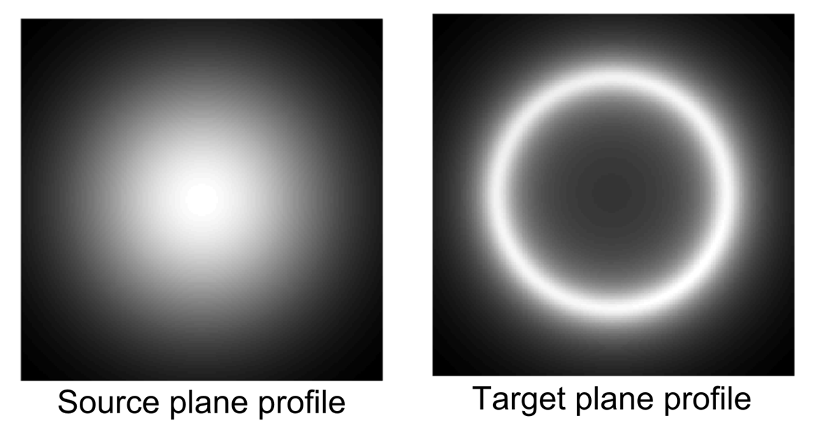
In 2016, I and some people in Oxford and Chicago realised that the shadowgraphy and proton radiography inverse problem is actually the optimal transport problem. The problem states more or less like “Given two density profiles (source and target profiles), determine the best way to move the densities from the source profile to form the target profile, so that the total distance travelled by the densities is minimised.” For simplicity, you can think the densities as pile of sand in the picture below.

The output of the problem stated above in this case is what I call as the deflection potential, \(\Phi\), which regulates the displacement from the source profile to the target profile as, \(\begin{equation} \mathbf{r}_{target} = \mathbf{r}_{source} - \nabla \Phi \end{equation}\) where \(\mathbf{r}\) is the position on source or target profile.
There have been a lot of algorithms to obtain the deflection potential from known source and target profiles. At the moment, my preference is from Sulman, et al. (2011), which was also used in Bott, et al. (2017). With some simple modification of the algorithm, we can cut down the run time from approximately 4 minutes to approximately 2-4 seconds (see the implementation in my GitHub repo).
Beyond shadowgraphy and proton radiography, we can use the code for other purposes. One of them is for “face interpolation”. Given two faces images, we can regard one of them as the source profile and the other one as the target profile. Putting them to the algorithm, we can obtain the deflection potential of those two faces, \(\Phi\). To interpolate the face, we can just multiply the deflection potential with some numbers and regard it as the deflection potential, i.e. \(\Phi\rightarrow\eta\Phi\), where \(\eta=[0,1]\).
Here are the two faces images I got from the internet.

There is no special reason why I chose those faces. They were just chosen randomly from the internet. I don’t even know them.
As my algorithm implementation works best if the background is non-zero and equals to the mean value of the interesting part, I changed the background to gray image. Putting those two images into the algorithm, we can obtain the deflection potential. Multiplying the deflection potentials with \(\eta=[0,1]\), and get the faces, I obtained the animation below.

The face interpolation demo can be found in my GitHub repo in the demo_face_interpolation.m file.