How likely are Uber's autonomous vehicles safer?

Last week there was a tragic news of death by an Uber’s self-driving car. According to this news and the fatality report by IIHS, some estimated the probability of the crash happened if Uber’s autonomous vehicles (AV) are as safe as non-AV using negative exponential distribution. The answer is around 3\%, which can also happen by bad luck. Specifically, from the IIHS data, it was obtained there was 1 fatal crash for every 93 million miles travelled by non-AV cars (i.e. 34,439 fatal crashes in 3,220,667 million miles in the US). The author also extrapolated from a report by the time the crash happened (i.e. last week), Uber’s AV would have collected 3 million miles.

Using the same data, my question is slightly different, “how likely are Uber’s AV safer than non-AV on average?” To answer the question, we can use the Poisson distribution,

$$\begin{equation} \label{eq:poisson-distribution} P(k | \lambda) = \frac{\lambda^k e^{-\lambda}}{k!} \end{equation}$$

where $k$ is the number of occurrence and $\lambda$ is the expected number of occurrence. In 3 million miles travelled, the expected number of fatal crashes for non-AV is $\lambda_{nAV} \approx 3/93 \approx 0.0323$. The Uber AV would be safer if $\lambda_{AV} < \lambda_{nAV}$. Given the information that there is $k = 1$ fatal crash in 3 million miles for Uber AV, we can infer the expected number of occurrence with Bayesian inference,

$$\begin{equation} \label{eq:posterior-distribution} P(\lambda_{AV} | k) = \frac{P(k | \lambda_{AV}) P(\lambda_{AV})}{\int_0^\infty P(k | \lambda_{AV}) P(\lambda_{AV})\ \mathrm{d}\lambda_{AV}}. \end{equation}$$

The term $P(k|\lambda_{AV})$ is the Poisson distribution given in the equation $\ref{eq:poisson-distribution}$. The prior distribution can take different forms to capture our prior belief on how safe the AV is. As a general form, we can take the prior distribution to be

$$\begin{equation} \label{eq:prior-lambda} P(\lambda_{AV}) \propto \lambda_{AV}^p. \end{equation}$$

Putting the equation $\ref{eq:prior-lambda}$ to the equation $\ref{eq:posterior-distribution}$ with $k = 1$ gives us

$$\begin{equation} \label{eq:posterior-distribution2} P(\lambda_{AV} | k=1) = \frac{\lambda_{AV}^{1+p} e^{-\lambda_{AV}}}{\Gamma(p+2)} \end{equation}$$

where $\Gamma(z)$ is the gamma function.

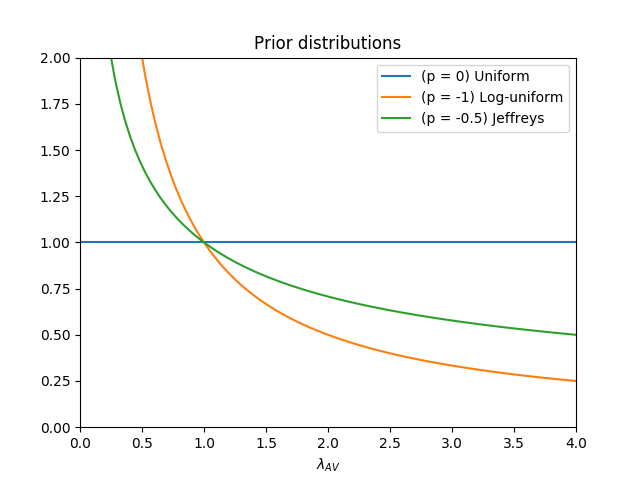
Let’s take 3 forms of prior distributions: (1) uniform, $p=0$, (2) log-uniform, $p = -1$, and (3) the Jeffreys prior for Poisson distribution, $p=-0.5$. The log-uniform and Jeffreys prior put a lot of belief of small $\lambda_{AV}$, which assumes the AV tends to be safe. Here is the plot of all prior distributions mentioned.

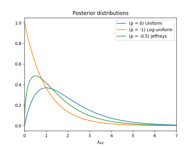
By substituting the values of $p$ to the posterior distribution equation $\ref{eq:posterior-distribution2}$, we can plot the posterior distribution of $\lambda_{AV}$ as shown in the figure below.

To calculate the likelihood it is safe, we can integrate the area under the curve for $\lambda_{AV} < \lambda_{nAV}$ with $\lambda_{nAV}\approx 0.0323$ from equation $\ref{eq:posterior-distribution2}$, which gives us

$$\begin{equation} \mathcal{L}(\lambda_{AV} < \lambda_{nAV}) = \int_0^{\lambda_{nAV}} P(\lambda_{AV} | k=1)\ \mathrm{d}\lambda_{AV} = 1 - \frac{\Gamma(p+2, \lambda_{nAV})}{\Gamma(p+2)} \end{equation}$$

where $\Gamma(z,x)$ is the incomplete gamma function.

For uniform ($p=0$), log-uniform ($p=-1$), and Jeffreys ($p=-0.5)$ priors, the likelihood of Uber AV being safer than non-AV respectively are $0.00051$, $0.032$, and $0.0043$. From these calculation, we can see even if we have strong prior that the Uber AV is safer (i.e. log-uniform prior), there still a small chance $3.2\%$ of the Uber AV is now safer than non-AV. Personally I would prefer Jeffreys prior as it is invariant under re-parameterization, so I belief that only miniscule chance, $0.43\%$, that Uber AV is safer, which means the non-AV is almost certainly safer than Uber AV, for now. I believe (and hope) Uber will improve to reduce the expected number of fatal crashes in the future.