Optimal transport for A/B test

This post was inspired by a post in Uber engineering blog. In the post, they talk about using Quantile Treatment Effect (QTE) to get more insights of an experiment. Here, I will talk about the similar case, with the same method, but from different perspective: optimal transport.

Case study: an A/B test example

Consider a case where you are testing a new design for your website to increase the time visitors spend on your website (i.e. online time). To test the new design, you set the website to show the new design to some proportion of the visitors, say 1%, and collect the online time for those who get the new design and those who get the old design (i.e. control). Let’s say you obtain an histogram as shown below.

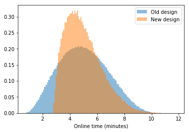
The question is: if the new design is implemented, how many visitors will spend longer time and how many visitors will spend shorter time, compared to the old design?

In the Uber’s blog post, they can get this insight by applying Quantile Treatment Effect (QTE). As we will see later, this is actually equivalent to a well-studied field called optimal transport, with a lot more properties.

Optimal transport

The first known formalization about optimal transport is by G. Monge in 1781. He posed a problem on how to optimally transport resources from a set of mines (i.e. sources) to the places that need them (i.e. targets). Optimally transport could mean minimizing the total distance travelled to distribute the materials or minimizing some cost function.

Despite the simplicity of the problem, the application is actually very vast. One very obvious application is in economics to optimally distribute resources. Not very obvious one is to design glass surface to get Alan Turing’s face on a wall (link). I have also posted an application of optimal transport for face interpolation and publish a paper to invert the integrated magnetic field from proton radiography (paper).

Optimal transport in 1D

A simple algorithm can be used to solve the optimal transport in 1D, i.e. if the sources and the targets are in a line, and the cost of transportation between two points is simply quadratic of the distance.

Let’s say the number of sources per unit length in a certain position \(x\) is \(\rho_s(x)\) and the number of targets per unit length is \(\rho_t(x)\). The total number of sources is assumed to be equal to the total number of targets, i.e.

The optimal transport with quadratic distance is solving (don’t worry about the equation, it’s totally fine if you don’t understand it)

The integrand above is the amount of work required to move a small amount of source, \(\rho_s dx\), from \(x\) to \(T(x)\), and the constraint is just enforcing the mass conservation.

To solve this, first let’s define the cumulative function of the sources and the targets as

One can obtain the optimal transport function, \(T(x)\), by calculating

i.e. by getting the position in the target cumulative function with the same quantile.

This is the same method with what is shown in the Uber’s post about QTE, we just approach it from different perspective.

Optimal transport for the A/B test

Let’s go back to our test case and let’s answer the question on the first section. If you’d like to replicate the result, the synthetic data can be downloaded from here for the control and from here for the new design. In this section, we will use the Python Optimal Transport library (POT).

First thing to do is, of course, load the data.

import numpy as np
from scipy.spatial.distance import cdist
import matplotlib.pyplot as plt
import ot

# load the data
samples_old = np.loadtxt("control.txt")
samples_new = np.loadtxt("new.txt")

For the optimal transport to work, we need to bin the samples into histograms.

nbins = 100
yhist_old, xhist_old = np.histogram(samples_old, bins=nbins)
yhist_new, xhist_new = np.histogram(samples_new, bins=nbins)

# normalization
yhist_old = yhist_old * 1.0 / np.sum(yhist_old)
yhist_new = yhist_new * 1.0 / np.sum(yhist_new)

# get the centre of the bins
xhist_old = (xhist_old[1:] + xhist_old[:-1]) / 2.0
xhist_new = (xhist_new[1:] + xhist_new[:-1]) / 2.0

One important thing is that the histogram must be normalized to the same total density, hence the normalization in the code above.

Now, we are ready to solve the optimal transport problem.

# get the distance matrix
M = cdist(xhist_old[:,None], xhist_new[:,None], "sqeuclidean")

# compute the transport matrix
T = ot.emd(yhist_old, yhist_new, M)

The transport matrix, T, is given as a matrix with \((i,j)\) element represents the amount of source \(i\) go to the target \(j\).

Given the transport matrix, we can visualize which element in the sources go to which element in the targets.

Tnorm = T / np.sum(T,axis=1)[:,None] # row normalization
xt = np.matmul(Tnorm, xhist_new[:,None]).flatten()
plt.plot(xhist_old, xt)
plt.plot(xhist_old, xhist_old, '--')
plt.xlabel("Original online time")
plt.ylabel("New online time")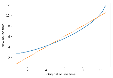

The normalization T / np.sum(T,axis=1)[:,None] was done to make the sum of each row of T to 1. This means the \((i,j)\) element in T represents the percentage of source \(i\) that goes to the target \(j\).

Now we can plot the quantile vs the displacement.

qtile = np.cumsum(yhist_old)
displacement = xt - xhist_old
plt.plot(qtile, displacement)
plt.plot(qtile, np.zeros_like(qtile), '--')
plt.xlabel("Visitors quantile")
plt.ylabel("Online time increment")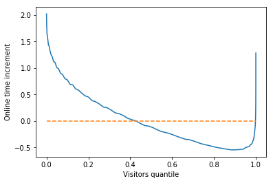

We can see there is about 40% of the visitors would have longer online time and 60% would have shorter online time, from this synthetic data. We can also see that the visitors with less online time on the old design tends to have more online time on the new design. Is the new design better or worse? It depends on the business case.

Uncertainties

The optimal transport (and equivalently, QTE) above would be correct if we assume the order of visitors according to the online time does not change, i.e. if A has longer online time than B with the old design, then A also has longer online time than B with the new design. This is not necessarily true in real life.

With optimal transport, there is a way to incorporate this type of uncertainty using entropy regularization.

reg = 0.5 # regularization factor
Treg = ot.sinkhorn(yhist_old, yhist_new, M, reg)

Higher regularization factor means it deviates more from the assumption. The amount of regularization factor depends on your “belief” on how much it deviates the same-order assumption. Another experiment might be necessary if you really want to get a good regularization factor.

Treg_norm = Treg / np.sum(Treg, axis=1)[:,None]
xreg_t_mean = np.matmul(Treg_norm, xhist_new[:,None]).flatten()
xreg_t_var = np.matmul(Treg_norm, (xhist_new-xreg_t_mean)[:,None]** 2).flatten()
xreg_t_std = np.sqrt(xreg_t_var)

# plot
plt.plot(xhist_old, xreg_t_mean)
plt.fill_between(xhist_old, xreg_t_mean-xreg_t_std,
                 xreg_t_mean+xreg_t_std, alpha=0.2)
plt.plot(xhist_old, xhist_old, '--')
plt.xlabel("Original online time")
plt.ylabel("New online time")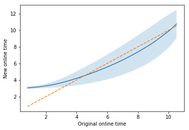

Now, the quantile vs online time with uncertainty.

displacement_mean = xreg_t_mean - xhist_old
plt.plot(qtile, displacement_mean)
plt.fill_between(qtile, displacement_mean - xreg_t_std,
                 displacement_mean + xreg_t_std, alpha=0.2)
plt.plot(qtile, np.zeros_like(qtile), '--')
plt.xlabel("Visitors quantile")
plt.ylabel("Online time increment")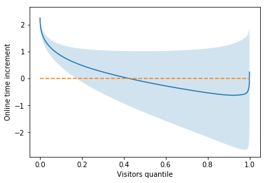

Here we can see a new insight by incorporating the uncertainty: the least-engaged visitors almost surely spend more time with the new design. This insight cannot be obtained if we just see the average of the distribution and without incorporating the uncertainty in the quantile analysis.

Conclusions

We have seen here that optimal transport can be used to analyze A/B testing results. Optimal transport in 1D is actually equivalent to QTE. Seeing it as an optimal transport problem opens up a lot of tools to analyze the results (e.g. entropy regularization).

The notebook for this post can be found here