Estimating the case survival rate from COVID19 in Indonesia
Summary
Using a model that takes into account delay in recovery and death, I calculate there is a 71% chance of survival from the confirmed case. This does not mean that there is a 71% chance of survival if infected by the virus, but this means, with the current government testing scheme, there is a 71% chance of survival if the government confirms positive. The low number of case survival rate could indicate that the current reported number of confirmed cases is heavily disproportionate towards the severe cases.
Introduction
With almost all parts of the world is observing the outbreak of COVID19, one thing that worries me is the situation in my home country, Indonesia. As of 24 March 2020, there are 686 patients confirmed to have the nCov-2019. Worryingly, out of 85 patients that have outcomes, there are 65% death cases (55 patients) and 35% of the patients recovered (30 patients). However, the 35% should not be taken as the case survival rate as it might take longer for the survived patients to be declared as fully recovered than the deceased patients to be declared as deceased.
Another way to estimate the death rate is by dividing the current accumulated deceased patients with the total confirmed case. This way, we get an estimate of 92% case survival rate (i.e. 1 - 55/686). Unfortunately, the number might not be accurate because not every active case will end up being recovered.
This naturally raises a question: can we estimate the case survival rate from the early outbreak data?
Model
Estimating the case survival rate from the early outbreak data requires some assumption to build a mathematical model and fit the model to the data. From the fitting result, one can then infer the estimated case survival rate.
The model I am using here is a modified SEIR model, but with splitting paths ending up in recovery and death. Here is the schematics of the model:

The states of people in the model are:
Susceptible: general population who can be infected by the virus.Exposed: people who already contracted the virus, but not developed the symptoms yet.Infectious: people who have already developed the symptoms and can infect others.Isolated 1: people who have been confirmed to have to have the virus and isolated.Isolated 2: same as isolated 2, but will recover eventually.Deceased: people who have died due to the virus.Recovered: people who have recovered from the disease.
The confirmed case is assumed to be number of people in states Isolated 1 and
Isolated 2.
To describe the transition between the states, I used several variables:
- \(r_{inf}\) (infection rate): how likely a person to infect a healthy person in a day.
- \(\tau_{incub}\) (incubation period): how long the virus takes to develop the symptoms and make the infected person infectious.
- \(\tau_{conf}\) (Confirmed period): how long it takes for a person to be confirmed positive once developed the symptoms.
- \(\tau_{dec}\) (Deceased period): how long it takes from being confirmed to be deceased (if they will).
- \(\tau_{rec}\) (Recovery period): how many days from being confirmed to be recovered (if they will).
- \(\eta\) (Case survival rate): the chance of a patient confirmed to have the virus to be recovered.
If we know the parameters above and the initial condition, we can predict how many people in every state (e.g. how many infectious people in a given time). However, we don’t know those parameters and we can get the data on how many people in some states from publicly available data. Therefore, we can infer the parameters above to match the observed data. In this case, we use the data of confirmed case, accumulated death number, and accumulated recovery number when the growing is exponential.
Mathematical detail
(If you are not interested in the mathematical details, you can skip this section)
Let’s denote the number of people in the Exposed state as \(n_e\),
Infectious as \(n_{if}\), Isolated 1 as \(n_{is1}\), Isolated 2 as
\(n_{is2}\), Deceased as \(n_d\), and Recovered as \(n_r\).
The dynamics of the states can be written as series of ordinary differential
equations (ODE):
As matrix, it can be written as
\[\begin{equation} \frac{\partial}{\partial t}\begin{pmatrix} n_e \\ n_{if} \\ n_{is1} \\ n_{is2} \\ n_{dec} \\ n_{rec} \end{pmatrix} = \mathbf{K} \begin{pmatrix} n_e \\ n_{if} \\ n_{is1} \\ n_{is2} \\ n_{dec} \\ n_{rec} \end{pmatrix} \end{equation}\]where
\[\begin{equation} \mathbf{K} = \begin{pmatrix} -\frac{1}{\tau_{incub}} & r_{inf} & 0 & 0 & 0 & 0 \\ \frac{1}{\tau_{incub}} & -\frac{1}{\tau_{conf}} & 0 & 0 & 0 & 0 \\ 0 & \frac{1-\eta}{\tau_{conf}} & -\frac{1}{\tau_{dec}} & 0 & 0 & 0 \\ 0 & \frac{\eta}{\tau_{conf}} & 0 & -\frac{1}{\tau_{rec}} & 0 & 0 \\ 0 & 0 & \frac{1}{\tau_{dec}} & 0 & 0 & 0 \\ 0 & 0 & 0 & \frac{1}{\tau_{rec}} & 0 & 0 \end{pmatrix} \end{equation}\]One of the solution of the equation above is \(n_{\cdot}(t) = n_{\cdot 0}e^{\kappa t}\) where \(n_{\cdot 0}\) is the number of people in some states at the initial time, and \(\kappa\) is the exponential factor. The exponential factor, \(\kappa\), is the largest eigenvalues of the matrix \(\mathbf{K}\). It can also be inferred from the data by performing linear fit of the logarithm of confirmed case versus time.
The ratio of the number of people in every states can be determined based on the eigenvector of the matrix \(\mathbf{K}\) that corresponds to the largest eigenvalue. The calculated ratio can then be compared with the data.
Fitting process
The model and assumption above is more accurate when the growing is still exponential and the number is not that small to avoid large statistical error. The observables that I use in this case are:
- Gradient of logarithm of confirmed case: \(\kappa\)
- Ratio between the deceased and the confirmed case: \(n_{dec} / (n_{is1}+n_{is2})\)
- Ratio between the deceased and the recovered patients: \(n_{dec} / n_{rec}\)
I took the mean and the standard deviation of every observable and assume to have a normal distribution. The fitting process is then proceeded by finding the posterior distribution of all parameters which can be retrieved with Markov Chain Monte Carlo (MCMC).
As there are more parameters to be inferred (i.e. 6) than the number of observables (i.e. 3), more constraints are needed to restrict the inferred parameters to have meaningful value. One constraint is applied by restricting the basic reproduction number (\(R_0\)) to be less than 4 from various estimate.
Results
Validation using data from China
To verify the model, we need data that shows exponential growing at the beginning of the outbreak and stabilize at the end to know the actual survival rate. The only country that satisfies this requirement is China. We took the data from here and took the data from 22-28 January 2020 as the exponential growing part. From the current data, the case survival rate is about 95.7%.
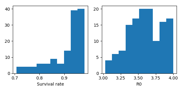
Based on the model above, we drew 1,000 samples from the posterior distribution using Markov Chain Monte Carlo. Here is the posterior distribution of the case survival rate and the basic reproduction rate (\(R_0\)) after constraining \(R_0\) to be less than 4.

We can see that the posterior distribution of the case survival rate in China is \(\eta = 94^{+2}_{-10}\%\), which is really close to the current number (\(95.7\%\))
Case survival rate estimation in Indonesia
After a simple validation of the model on China’s data, I applied the same technique for Indonesia. Here I took the data from 18-24 March 2020 because it shows approximately exponential growth and the ratios are more or less constant.
Other than constraining the \(R_0\) to be less than 4, I also constraint the deceased period (\(\tau_{dec}\)) to be between 9 and 13 days. This estimate was obtained from table compiled by KawalCOVID19.
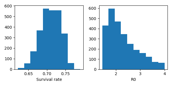
From the sampled posterior distribution and the constraints, here is the posterior distribution of the case survival rate in Indonesia.

As seen in the Figure above, the case survival rate in Indonesia is approximately \(\eta = 71^{+3}_{-3}\%\), which is worryingly low. This does not mean that there is a 71% chance of survival if infected by the virus, but this mean, with the current government testing scheme, there is 71% chance of survival if the government confirms positive.
Caveats
The numbers above should be taken with several caveats:
-
The case survival rate depends heavily on the estimated deceased period (i.e. the time a person to be deceased after being confirmed). For example, constraining the deceased period to be between 1 to 4 days gives the case survival rate about 88%. As the data to estimate this parameter is very hard to obtain, I estimate it from the current status of the first 450 patients. I assume the order of death is based on the order of confirmation (e.g. patient 71 gets deceased before 72 & 74). If the assumption is very much off, then the estimated deceased period could be really off.
-
I made several assumptions in building the model to keep it simple. If the assumption is wrong, then the model is wrong, hence the number is wrong.
-
Based on the posterior distribution from Indonesia’s data, it is estimated that the recovery time can be 2 months, which is very long. This might be the sign that the model cannot explain fully the data.
-
The number of recovered patients are still quite low (i.e. 30 as of 24 March 2020), so it might be prone to statistical noise.
Code availability
The code is available here with BSD 3-clause license.
Update history
Update 25/03/2020: adding summary and making clear about the number interpretation