Score-based generative model tutorial 1st part: without SDE

This is 2 part tutorials where the second part can be found here. The jupyter notebooks for this tutorial can be found here.

Generative model

If you’ve had too much time on the internet lately, you probably have seen the text-to-image generators such as DALL-E 2, Imagen, or CogView2. One of the key building blocks of those systems is the generative model. Generative model is the part responsible to generate images that looks as realistic as possible.

How does a generative model works? The generative model is trained with a set of real data (or image) as its training dataset. Statistically speaking, the training dataset can be seen as data sampled from an unknown probability distribution. During the training, this distribution is to be unveiled and if the training is successful, the generative model can sample new data from this distribution.

The details on how a generative model unveil the distribution and sample data from this distribution are different based on the type of the generative model. One class that I would like to talk in this series of blog posts is the score-based generative model with stochastic differential equations, based on this paper.

Score-based generative model (without SDE)

Before continue reading this post, I highly recommend reading the great blog post about score-based generative model by Yang Song here to understand the basic of score-based generative model.

Let’s denote the real data (e.g. images, videos) as \(\mathbf{x}\in\mathbb{R}^n\) as a vector of \(n\) elements. For example, if we are working with MNIST images i.e. grey-scale image (1 channel) with 28-by-28 pixels, the value of \(n\) would be \(n=1\times 28\times 28=784\). The training data, \(\mathbf{x}_{1..N}\), is assumed to be drawn from an unknown probability distribution function, \(p(\mathbf{x})\), i.e. \(\mathbf{x}\sim p(\mathbf{x})\).

What we want to learn in score-based generative model is the score function (i.e. gradients of log probability density function), \(\nabla_\mathbf{x} \mathrm{log}\ p(\mathbf{x})\), given samples of the training data, \(\mathbf{x}_{1..N}\). By learning the score function, we can sample from the distribution using sampling algorithms, such as Langevin MCMC. Learning the score function does not have any constraint as opposed to learning the probability density function where we have to make sure the total integral is 1. Having the total integral constraint removed in score-based generative model, we get more freedom in choosing the architecture of the neural network.

The learned score function \(\mathbf{s}(\mathbf{x};\theta)\) can be represented by a neural network that takes the data \(\mathbf{x}\) as the input and produces an output with the same size as its input. The neural network’s parameters, \(\theta\), can be learned by minimizing the loss function with respect to the true score function \(\nabla_\mathbf{x} \mathrm{log}\ p(\mathbf{x})\),

where the expectation value \( \mathbb{E}_{\mathbf{x}\sim p(\mathbf{x})}\left[\cdot \right] \) can be obtained by calculating the mean of the term inside the bracket using the training data. However, in a usual setting, the true gradients of the log probability density functions \(\nabla_{\mathbf{x}} \mathrm{log}\ p(\mathbf{x})\) are not available in the training data. Hyvarinen (2005) shows that the loss function above can be rewritten as

In the equation above, only the first and second terms need to be computed during the training. The term \(g(\mathbf{x})\) does not depend on the neural network parameters, \(\theta\), so it does not matter in the optimization of \(\theta\). The first term is simply half of the vector norm of the score function while the second term, \(\mathrm{tr}\left(\nabla_\mathbf{x} \mathbf{s}(\mathbf{x}; \theta)\right)\), is the trace (i.e. sum of the diagonal) of the Jacobian matrix \(\nabla_\mathbf{x} \mathbf{s}(\mathbf{x}; \theta)\).

Implementation

Let’s take a simple dataset where the data \(\mathbf{x}\) is a vector of 2 elements generated from the swiss roll distribution.

import torch
from sklearn.datasets import make_swiss_roll

# generate the swiss roll dataset
xnp, _ = make_swiss_roll(1000, noise=1.0)
xtns = torch.as_tensor(xnp[:, [0, 2]] / 10.0, dtype=torch.float32)
dset = torch.utils.data.TensorDataset(xtns)

Now let’s define the neural network that will learn the score function. This is just a simple multi-layer perceptron with LogSigmoid activation function. I used LogSigmoid because of personal preference, you can also use ReLU.

# score_network takes input of 2 dimension and returns the output of the same size
score_network = torch.nn.Sequential(
    torch.nn.Linear(2, 64),
    torch.nn.LogSigmoid(),
    torch.nn.Linear(64, 64),
    torch.nn.LogSigmoid(),
    torch.nn.Linear(64, 64),
    torch.nn.LogSigmoid(),
    torch.nn.Linear(64, 2),
)

After that, we can implement the first and second terms of the loss function below,

Note that to implement the Jacobian, we can use the functions from functorch.

from functorch import jacrev, vmap

def calc_loss(score_network: torch.nn.Module, x: torch.Tensor) -> torch.Tensor:
    # x: (batch_size, 2) is the training data
    score = score_network(x)  # score: (batch_size, 2)
    
    # first term: half of the squared norm
    term1 = torch.linalg.norm(score, dim=-1) ** 2 * 0.5
    
    # second term: trace of the Jacobian
    jac = vmap(jacrev(score_network))(x)  # (batch_size, 2, 2)
    term2 = torch.einsum("bii->b", jac)  # compute the trace
    return (term1 + term2).mean()

Everything is ready, now we can start the training. In my computer, it takes about 10-15 minutes to finish.

# start the training loop
opt = torch.optim.Adam(score_network.parameters(), lr=3e-4)
dloader = torch.utils.data.DataLoader(dset, batch_size=32, shuffle=True)
for i_epoch in range(5000):
    for data, in dloader:
        # training step
        opt.zero_grad()
        loss = calc_loss(score_network, data)
        loss.backward()
        opt.step()

Once the neural network is trained, we can generate the samples using Langevin MCMC.

where \(\mathbf{z}_i\sim\mathcal{N}(\mathbf{0}, \mathbf{I})\) is a random number sampled from the normal distribution.

def generate_samples(score_net: torch.nn.Module, nsamples: int, eps: float = 0.001, nsteps: int = 1000) -> torch.Tensor:
    # generate samples using Langevin MCMC
    # x0: (sample_size, nch)
    x0 = torch.rand((nsamples, 2)) * 2 - 1
    for i in range(nsteps):
        z = torch.randn_like(x0)
        x0 = x0 + eps * score_net(x0) + (2 * eps) ** 0.5 * z
    return x0

samples = generate_samples(score_network, 1000).detach()

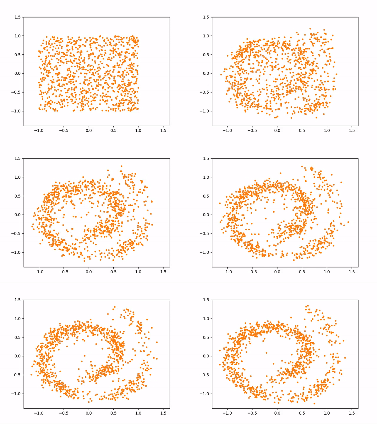
The sampling process above more or less looks like below:

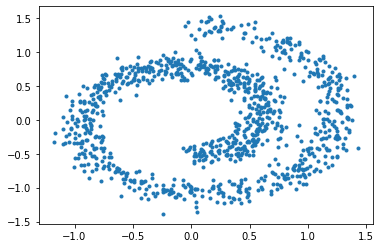
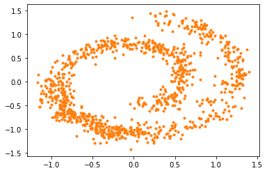
And here are the samples from our trained model on the left, compared to the training samples on the right:

As we can see, the generative model can draw new samples from the swiss dataset without knowing the distribution explicitly. However, there are several discrepancies, like our generative model generates more samples on the bottom left than it should be. In the next tutorial, we will go through how to improve the sampling quality by using stochastic differential equations (SDE).

Summary

Summary for this part:

• Neural network: \(n\) input parameters, \(\mathbf{x}\), with \(n\) output parameters, \(\mathbf{s}(\mathbf{x};\theta)\).
• Training: minimize \(\mathcal{L}(\theta) = \mathbb{E}_{\mathbf{x}\sim p(\mathbf{x})}\left[\frac{1}{2} \left\lVert\mathbf{s}(\mathbf{x};\theta)\right\rVert^2 + \mathrm{tr}\left(\nabla_\mathbf{x} \mathbf{s}(\mathbf{x}; \theta)\right)\right].\)
• Samples generation: \(\mathbf{x}_{i + 1} = \mathbf{x}_i + \varepsilon \mathbf{s}(\mathbf{x}; \theta) + \sqrt{2\varepsilon} \mathbf{z}_i\) for \(i=\{0, …, N\}.\) with \(\mathbf{z}_i\sim \mathcal{N}(\mathbf{0}, \mathbf{I})\) and some small value of \(\varepsilon\) and reasonable value of \(\mathbf{x}_0\).

The jupyter notebook for this tutorial can be found here. Continue to the 2nd part.