Score-based generative model tutorial 2nd part: with SDE

This is a 2 part tutorial of score-based generative model based on this paper. The first part of the tutorial can be read here. By the end of this tutorial, hopefully you can learn how to generate MNIST images. The jupyter notebooks for this tutorial can be found here.

Why using SDE?

In the previous tutorial, we’ve talked about the basic implementation of score-based generative model (SGM) without the stochastic differential equation (SDE) part. In that post, it works well even without SDE because it only has a small number of parameters (i.e. 2).

The drawback of the method in the previous tutorial is that it cannot learn the score function (i.e. the gradient of log probability density function) in the region where there are less training samples. It can only learn accurate score function where there are a lot of training samples. Yang Song’s blog post brilliantly illustrate and explain this.

This is problematic in generating the samples using Langevin MCMC. If we start the samples in the region where the score function is less accurate, the Langevin MCMC might not generate the samples with the correct distribution. We can see this effect in the animation below.

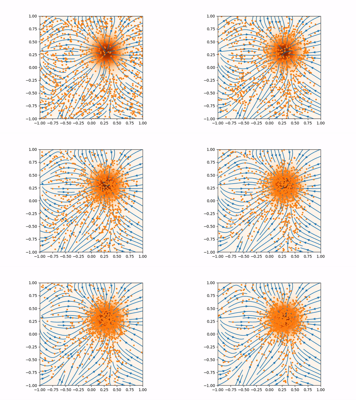
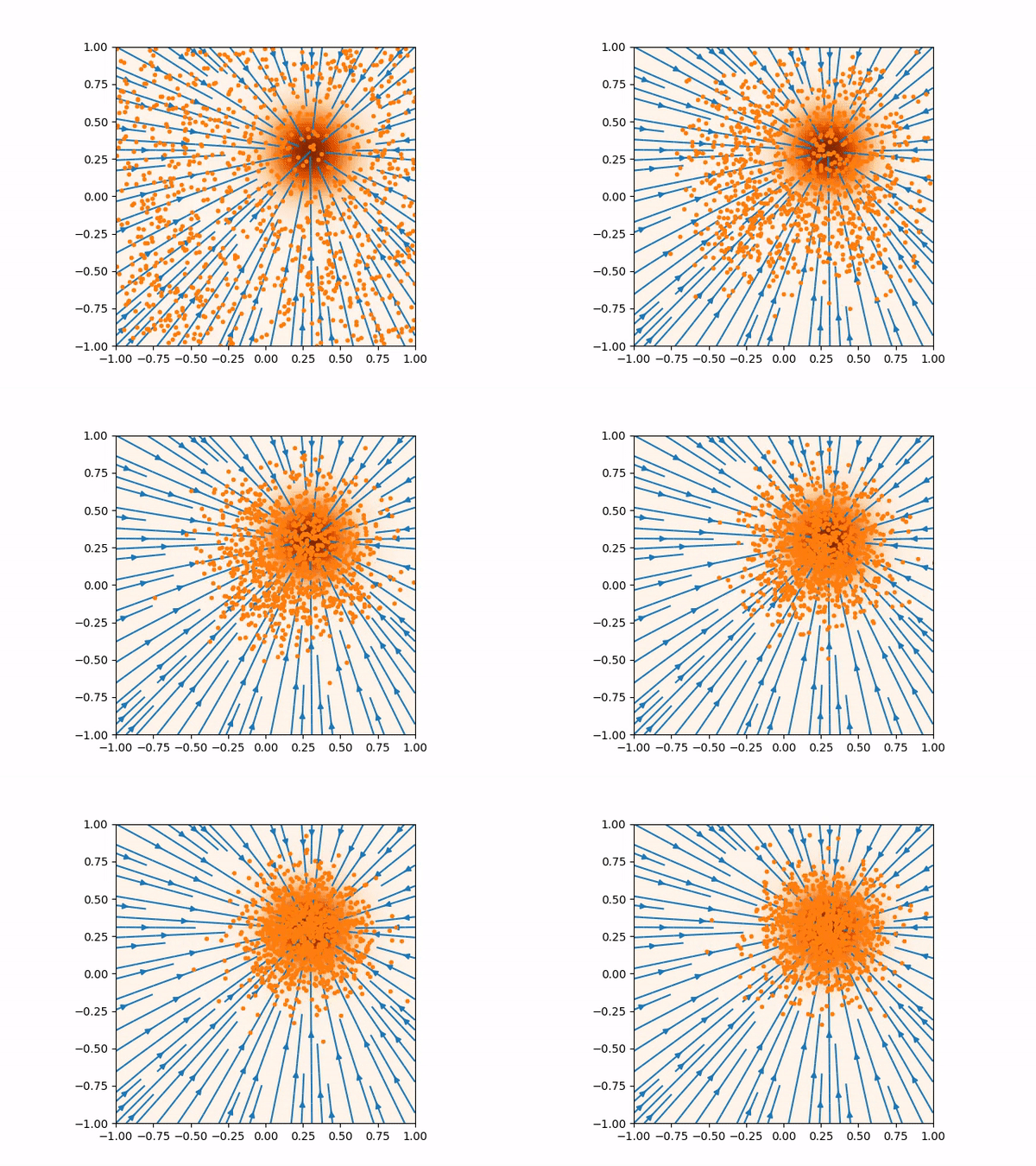
(Left) Inaccurate score function far from the training data would produce bad sampling. (Right) This is how the score function and the sampling should be.

One way to solve this problem is to “evolve” the true distribution into some known distribution, like normal distribution. If the evolution is smooth enough, we can start by sampling the normal distribution, then slowly backtrack the evolution back into the true distribution. This way, we don’t need accurate score function in the region where there are less samples because we can guide the samples to be close to the true distribution by backtracking the evolution of the distribution.

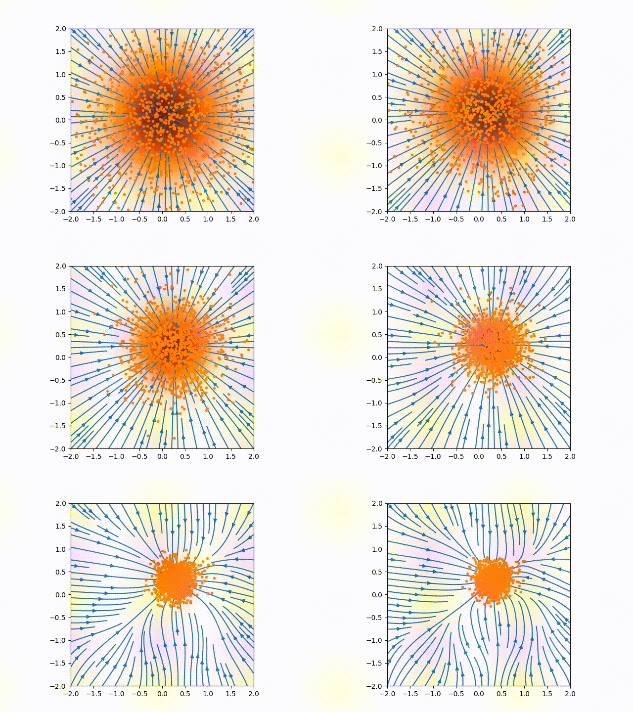
By having the distribution evolving, we can correctly sample without having to make the score function accurate everywhere

Mathematically, the probability distribution function of the samples now depends on an additional variable, for example, the evolution time \(t\), i.e. \(p(\mathbf{x}, t)\) where \(p(\mathbf{x}, 0)\) is the true distribution and \(p(\mathbf{x}, T)\approx\mathcal{N}(\mathbf{0}, \mathbf{I})\) to allow easy sampling at \(t=T\) (we can take \(T = 1\)).

This is the role of the stochastic differential equation (SDE): to provide the evolution path from the true distribution to a normal distribution. Specifically, if our signal is written as \(\mathbf{x}\), the evolution of the signal along the time \(t\) can be written as

where \(\mathbf{f}(\mathbf{x}, t)\) is the drift term and \(g(t)\) is the diffusion term. Knowing the drift and diffusion terms as well as the initial signal \(\mathbf{x}(0)\), it is possible to calculate the solution \(\mathbf{x}(t)\) numerically. For example, by using Euler-Maruyama algorithm, the update step is given by

There are various ways to define the drift and diffusion terms, but here we just pick one way that is known as the Variance Preserving with

Here we choose \(\beta(t) = 0.1 + (20 - 0.1) t\) with the evolution goes from \(t = 0\) to \(t = 1\). The values chosen here would produce the distribution of \(\mathbf{x}(t)\) at \(t=1\) close to the normal distribution.

Training with SDE

With the evolution of the distribution along the time \(t\), our neural network should accept the signal \(\mathbf{x}\) and the time \(t\) as its input parameters and produce the score function, i.e. \(\mathbf{s}(\mathbf{x}, t; \theta)\) with \(\theta\) as its parameters. The shape of the neural network output \(\mathbf{s}\) should be the same as the signal \(\mathbf{x}\). In this case, the denoising score matching loss function can be used

where \(\lambda(t)\) is the custom loss weighting function. For this case, we can choose \(\lambda(t) = 1-e^{\int_0^t \beta(s)\ ds}\). Another term in the loss function above is the posterior distribution function, \(p(\mathbf{x}(t)|\mathbf{x}(0))\). Fortunately, because we know the diffusion and drift terms in the SDE above, the posterior distribution function can be written analytically as

where

Therefore,

The ability to compute the posterior distribution function analytically is a big advantage. This means that we don’t have to solve the SDE numerically during the training. This makes the training for score-based generative model with SDE relatively fast.

Sampling with reverse SDE

Because of the chosen SDE drift and diffusion terms above, the distribution of \(\mathbf{x}(1)\) will be close to the normal distribution, i.e. \(p(\mathbf{x}(1))\approx\mathcal{N}(\mathbf{0}, \mathbf{I})\). Therefore, it is easy to draw samples of \(\mathbf{x}(1)\). However, we are interested in the true distribution of the training data, or \(\mathbf{x}(0)\). As \(\mathbf{x}(1)\) can be obtained by solving the SDE above from \(\mathbf{x}(0)\), the variable \(\mathbf{x}(0)\) can be obtained from \(\mathbf{x}(1)\) by solving the reverse SDE,

where \(\mathbf{s}(\mathbf{x}, t; \theta)\) is the learned score function from the training, \(\mathbf{f}(\mathbf{x}, t)\) and \(g(t)\) are respectively the drift and diffusion terms from the forward SDE above.

Implementation

Similar to the previous part, let’s take a simple example of generating swiss roll dataset.

import torch
from sklearn.datasets import make_swiss_roll

# generate the swiss roll dataset
xnp, _ = make_swiss_roll(1000, noise=1.0)
xtns = torch.as_tensor(xnp[:, [0, 2]] / 10.0, dtype=torch.float32)
dset = torch.utils.data.TensorDataset(xtns)

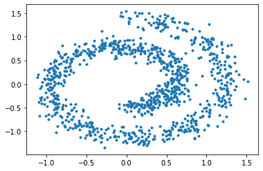
Now let’s define the neural network that will learn the score function. This is just a simple multi-layer perceptron with LogSigmoid activation function. In contrast to the previous part, the neural network here takes \(n + 1\) inputs and produces \(n\) outputs. The additional 1 input is for the time \(t\).

# score_network takes input of 2 + 1 (time) and returns the output of the same size (2)
score_network = torch.nn.Sequential(
    torch.nn.Linear(3, 64),
    torch.nn.LogSigmoid(),
    torch.nn.Linear(64, 64),
    torch.nn.LogSigmoid(),
    torch.nn.Linear(64, 64),
    torch.nn.LogSigmoid(),
    torch.nn.Linear(64, 2),
)

Now let’s implement the denoising score matching function below,

where \(\lambda(t) = 1 - \mathrm{exp}\left[-\int_0^t \beta(s) ds\right]\) and \(\nabla_{\mathbf{x}(0)}\mathrm{log}\ p(\mathbf{x}(t)|\mathbf{x}(0))\) can be calculated analytically,

with \(\beta(t) = 0.1 + (20 - 0.1) t\).

def calc_loss(score_network: torch.nn.Module, x: torch.Tensor) -> torch.Tensor:
    # x: (batch_size, 2) is the training data
    
    # sample the time
    t = torch.rand((x.shape[0], 1), dtype=x.dtype, device=x.device) * (1 - 1e-4) + 1e-4

    # calculate the terms for the posterior log distribution
    int_beta = (0.1 + 0.5 * (20 - 0.1) * t) * t  # integral of beta
    mu_t = x * torch.exp(-0.5 * int_beta)
    var_t = -torch.expm1(-int_beta)
    x_t = torch.randn_like(x) * var_t ** 0.5 + mu_t
    grad_log_p = -(x_t - mu_t) / var_t  # (batch_size, 2)
    
    # calculate the score function
    xt = torch.cat((x_t, t), dim=-1)  # (batch_size, 3)
    score = score_network(xt)  # score: (batch_size, 2)

    # calculate the loss function
    loss = (score - grad_log_p) ** 2
    lmbda_t = var_t
    weighted_loss = lmbda_t * loss
    return torch.mean(weighted_loss)

Everything’s ready, so we can start the training. In my computer, it takes about 20 - 25 minutes to complete the training. You can also add some progress checker (like tqdm) to see the progress.

# start the training loop
opt = torch.optim.Adam(score_network.parameters(), lr=3e-4)
dloader = torch.utils.data.DataLoader(dset, batch_size=256, shuffle=True)
for i_epoch in range(150000):
    for data, in dloader:
        # training step
        opt.zero_grad()
        loss = calc_loss(score_network, data)
        loss.backward()
        opt.step()

Once the neural network is trained, we can generate the samples using reverse SDE

where \(\mathbf{f}(\mathbf{x}, t) = -\frac{1}{2}\beta(t)\mathbf{x}\), \(g(t) = \sqrt{\beta(t)}\), and the integration time goes from 1 to 0. To solve the SDE, we can use the Euler-Maruyama method.

def generate_samples(score_network: torch.nn.Module, nsamples: int) -> torch.Tensor:
    x_t = torch.randn((nsamples, 2))  # (nsamples, 2)
    time_pts = torch.linspace(1, 0, 1000)  # (ntime_pts,)
    beta = lambda t: 0.1 + (20 - 0.1) * t
    for i in range(len(time_pts) - 1):
        t = time_pts[i]
        dt = time_pts[i + 1] - t

        # calculate the drift and diffusion terms
        fxt = -0.5 * beta(t) * x_t
        gt = beta(t) ** 0.5
        score = score_network(torch.cat((x_t, t.expand(x_t.shape[0], 1)), dim=-1)).detach()
        drift = fxt - gt * gt * score
        diffusion = gt

        # euler-maruyama step
        x_t = x_t + drift * dt + diffusion * torch.randn_like(x_t) * torch.abs(dt) ** 0.5
    return x_t

samples = generate_samples(score_network, 1000).detach()

The sampling process above more or less looks like below where you can see the evolution of the distribution from normal distribution to the true distribution of the training data.

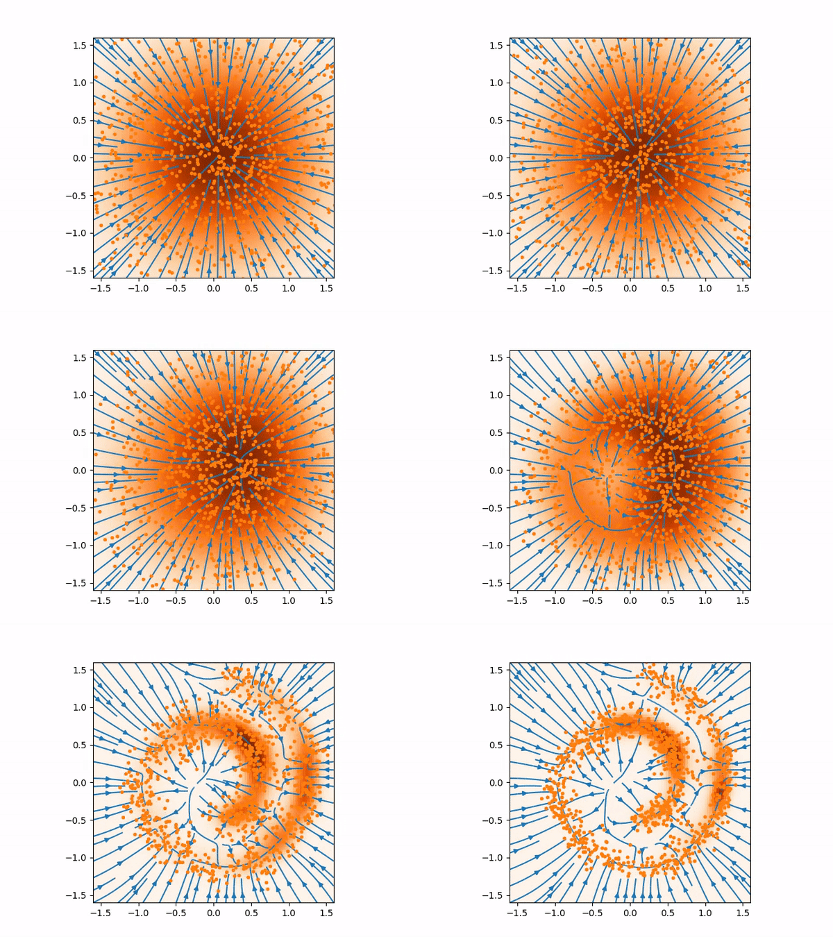
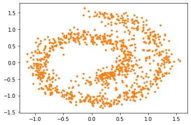
And here are the samples from our trained model on the left, compared to the training samples on the right:

The jupyter notebook going through the process above can be found here.

Generating MNIST

Once we’ve implemented the generative model for the example above, implementing it for image data is relatively straightforward. What we need to do is just to change the architecture of the score network into a U-Net architecture that takes the MNIST image of size \(28\times 28\) with 1 channel and the time \(t\), then produce the score function with the same shape as the MNIST image. To incorporate the time \(t\) into the architecture, I found that adding it as an additional channel in the input image works well (the additional channel will have all the same value as \(t\)). The architecture is illustrated below.

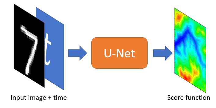
I have written a jupyter notebook here that goes through the training and generation. Most of the part is just the same as before with the only exception on the neural network architecture. After training it for 2 hours, here’s the results that we get.

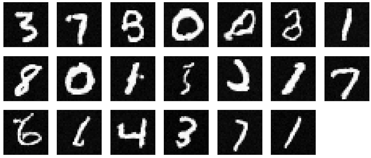
We can see that the generated image is relatively clean. However, there are some strange shapes that are generated. This is because in the example we’re using a relatively shallow U-Net architecture and only train it for about 400k training steps. We can improve this by having a better architecture (e.g. deeper U-Net) and train it for longer. If you have any other suggestions, please let me know.